|
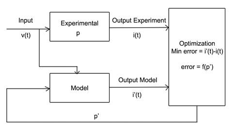
Model creation This document begins explaining the problem to solve to have a better understanding on how to create the models. Later the implementation for Pspice and Simulink is presented with an example for each. Problem explanationThe problem in mind can be represented as shown below. There is an experiment conducted where there are some parameters p that needs to be determined and are unknown. A model of the system is developed and is fed the same inputs. For the case where p’ is close to p the output of the experiment and the model will be similar. An error function is created between the different outputs of the model.
In the diagram above it is shown what could be the way to determine the parameters of an electrical machine. A set of voltages, v(t) are fed to the motor and the currents i(t) are recorded. Then the same voltages v(t) are given to a model where the parameters p’ can be varied. An objective function is created by comparing the outputs i(t) of model and experiment. As the parameters estimations p’ are closer to p the error decreases and the optimization can converge to a result that minimizes the error. All the problems to be solved are like this and the different implementation in Pspice and Simulink is shown later. It is important to understand that the model must receive the same inputs as the experiment and that the parameters to vary are what needs to be determined. If the model is not correctly designed you cannot expect correct results. The experiment inputs are designed within the model (for example the designing of v(t)) and the parameters p’ are left as inputs that the Optimization Tool can set. All the models will be created this way and the implementation in Pspice and Simulink is shown below. Pspice implementationAs stated before we must create a model that has the same inputs as the experiment and can provide outputs to be measured. The actual inputs of the model will be the parameters to vary. Below it is shown an IGBT dynamic turn-on/turn-off test model designed in Pspice.
The model performs a switching test on an igbt. The input can be considered the gate control and the outputs are the voltage Vce and the current trough the transistor over time, Ic. In order to let the Optimization Tool use this model we must specify the parameters and also write the outputs. ParametersTo specify a parameters simply add varParam(number) for as much parameters as you want. For the first one write varParam(1), for the second varParam(2) and so on. For example if we want to estimate the parameters: {t2, tb, t3, t4, gammab, gamma3, gamma2} Then we can modify the IGBT part where those parameters are present and we would put it as:
It is important from this point on that we follow the same order with the parameters if we need to have more simulations. Also, when we create the configuration file the same order must be maintain in the variables values and names. OutputsFinally you need to add a line telling Pspice to save the variables you want to have as outputs. For example in this circuit we want to have Vce = v(8)-v(9) and the current Ic = I(XDUT1:1). To do so we can simply add before the .end statement:
We must use the .print statement followed of the type of simulation. Usually it will be either dc or tran for steady-state values and transient phenomena respectively. It will be the same as the type of simulation ran. We can try to simulate the Pspice circuit (without the addition of parameters to determine with varParam()) and check in the .out file if the outputs are the desired. We must also know which output is which in the column later to specify the order in the Optimization tool. The circuit is now fully defined and will look like this after all the modifications:
If we run the Pspice file without the varParam() we can see in the middle of the .out file something like this:
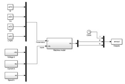
So we can see that the first column is the time, the second the voltage that we wanted and the third the current. In the optimization tool if we want to the curve v(8,9) = f(t) we would put 1 in xvar as it is the time and 2 in yvar as it is Vce. For the current it would be 1 and 3 respectively. Simulink implementationSimulink models may be a bit easier since are designed with blocks. ParametersEach parameter can be accessed in the model by referencing its position in a vector denoted as p using the same order as specified before with the varParam(). So to use the first parameter in the model simply write p(1) and for the second p(2) and so on. OutputsFor the outputs you must create a bus that has all the variables to save. You can add the clock block if you want to save the time also. The bus must converge to a “save to workspace” block with name “simout” and the save format must be “Timeseries”. An example with a PMSM is shown below:
The objective is to estimate the parameters: {R,Lq,Ld,Lmpm} They can be used in Simulink by calling its position in the p vector and are fed to the machine model. The voltages given in the experiment have been recorded and are given also to the model that will predict a current in d and q that is compared with the experimental one in Parameter Optimizer. The current and speed of the current period is also fed to the model because in this particular system the outputs depend of the previous instants and therefore a small error will pile up and produce wrong estimations so after each estimation of idq the program sets the previous current as the one from the experiment and not the actual predicted current. Parameter optimizer however will only see the model estimations. The outputs are the current in d and q and since we also want the time the clock block is added to the bus. Later in Parameter Optimizer to access the yvars for id we would put it as 2 as it is the second in the output and for iq a 3 since the time was set as the first. |

